Start at 2017-03-27 18:59:42
First, define topology of a map grid (2017-03-27 18:59:42)...
Second, initialise the codebook matrix (61 X 10) using 'linear' initialisation, given a topology and input data (2017-03-27 18:59:42)...
Third, get training at the rough stage (2017-03-27 18:59:42)...
1 out of 7 (2017-03-27 18:59:42)
updated (2017-03-27 18:59:42)
2 out of 7 (2017-03-27 18:59:42)
updated (2017-03-27 18:59:42)
3 out of 7 (2017-03-27 18:59:42)
updated (2017-03-27 18:59:42)
4 out of 7 (2017-03-27 18:59:42)
updated (2017-03-27 18:59:42)
5 out of 7 (2017-03-27 18:59:42)
updated (2017-03-27 18:59:42)
6 out of 7 (2017-03-27 18:59:42)
updated (2017-03-27 18:59:42)
7 out of 7 (2017-03-27 18:59:42)
updated (2017-03-27 18:59:42)
Fourth, get training at the finetune stage (2017-03-27 18:59:42)...
1 out of 25 (2017-03-27 18:59:42)
updated (2017-03-27 18:59:42)
2 out of 25 (2017-03-27 18:59:42)
updated (2017-03-27 18:59:42)
3 out of 25 (2017-03-27 18:59:42)
updated (2017-03-27 18:59:42)
4 out of 25 (2017-03-27 18:59:42)
updated (2017-03-27 18:59:42)
5 out of 25 (2017-03-27 18:59:42)
updated (2017-03-27 18:59:42)
6 out of 25 (2017-03-27 18:59:42)
updated (2017-03-27 18:59:42)
7 out of 25 (2017-03-27 18:59:42)
updated (2017-03-27 18:59:42)
8 out of 25 (2017-03-27 18:59:42)
updated (2017-03-27 18:59:42)
9 out of 25 (2017-03-27 18:59:42)
updated (2017-03-27 18:59:42)
10 out of 25 (2017-03-27 18:59:42)
updated (2017-03-27 18:59:42)
11 out of 25 (2017-03-27 18:59:42)
updated (2017-03-27 18:59:42)
12 out of 25 (2017-03-27 18:59:42)
updated (2017-03-27 18:59:42)
13 out of 25 (2017-03-27 18:59:42)
updated (2017-03-27 18:59:42)
14 out of 25 (2017-03-27 18:59:42)
updated (2017-03-27 18:59:42)
15 out of 25 (2017-03-27 18:59:42)
updated (2017-03-27 18:59:42)
16 out of 25 (2017-03-27 18:59:42)
updated (2017-03-27 18:59:42)
17 out of 25 (2017-03-27 18:59:42)
updated (2017-03-27 18:59:42)
18 out of 25 (2017-03-27 18:59:42)
updated (2017-03-27 18:59:42)
19 out of 25 (2017-03-27 18:59:42)
updated (2017-03-27 18:59:42)
20 out of 25 (2017-03-27 18:59:42)
updated (2017-03-27 18:59:42)
21 out of 25 (2017-03-27 18:59:42)
updated (2017-03-27 18:59:42)
22 out of 25 (2017-03-27 18:59:42)
updated (2017-03-27 18:59:42)
23 out of 25 (2017-03-27 18:59:42)
updated (2017-03-27 18:59:42)
24 out of 25 (2017-03-27 18:59:42)
updated (2017-03-27 18:59:42)
25 out of 25 (2017-03-27 18:59:42)
updated (2017-03-27 18:59:42)
Next, identify the best-matching hexagon/rectangle for the input data (2017-03-27 18:59:42)...
Finally, append the response data (hits and mqe) into the sMap object (2017-03-27 18:59:42)...
Below are the summaries of the training results:
dimension of input data: 100x10
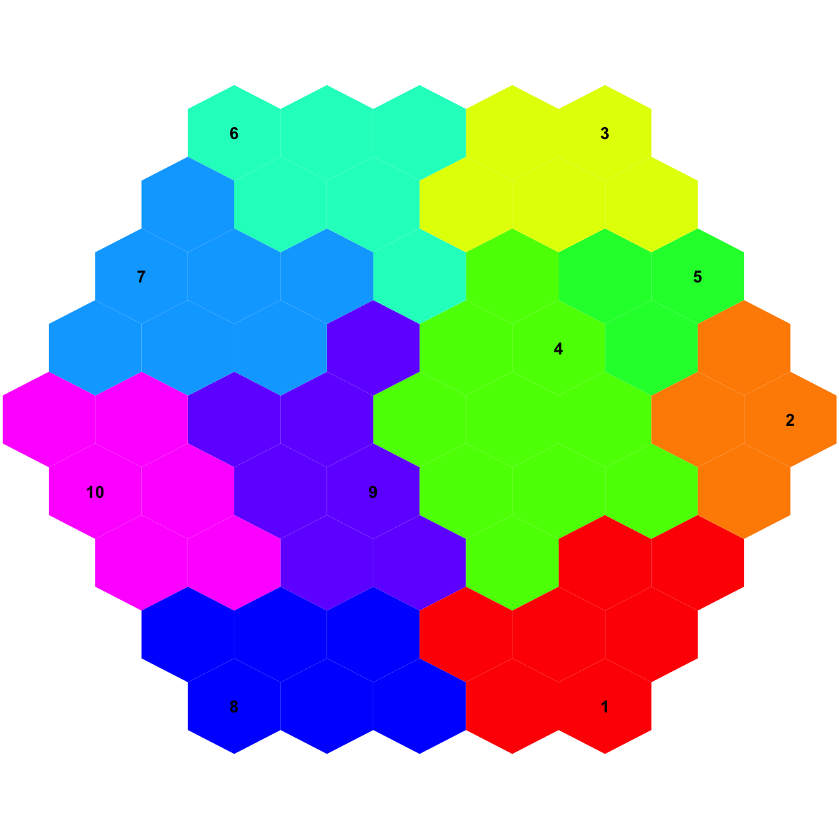
xy-dimension of map grid: xdim=9, ydim=9, r=5
grid lattice: hexa
grid shape: suprahex
dimension of grid coord: 61x2
initialisation method: linear
dimension of codebook matrix: 61x10
mean quantization error: 4.61431442408722
Below are the details of trainology:
training algorithm: batch
alpha type: invert
training neighborhood kernel: gaussian
trainlength (x input data length): 7 at rough stage; 25 at finetune stage
radius (at rough stage): from 3 to 1
radius (at finetune stage): from 1 to 1
End at 2017-03-27 18:59:42
Runtime in total is: 0 secs


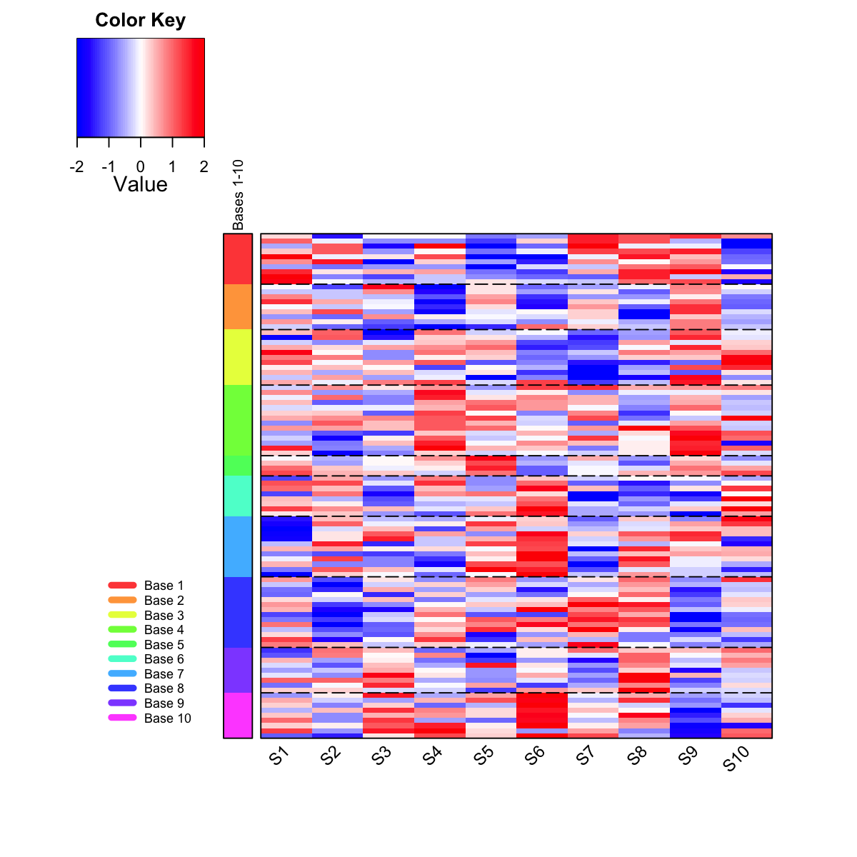
## As you have seen, heatmap is used to visualise patterns seen in genes within each meta-cluster/base. Row side bar indicates the meta-clusters/bases.
## The returned variable "output" (NOT a text file) has 1st column for your input data ID (an integer; otherwise the row names of input data matrix), and 2nd column for the corresponding index of best-matching hexagons (i.e. gene clusters), and 3rd column for the cluster bases (i.e. gene meta-clusters). Note: it has rows in the same order as visualised in the heatmap. You can save this output into the file 'output.txt':
write.table(output, file="output.txt", quote=F, row.names=F, sep="\t")

 ## As you have seen, heatmap is used to visualise patterns seen in genes within each meta-cluster/base. Row side bar indicates the meta-clusters/bases.
## The returned variable "output" (NOT a text file) has 1st column for your input data ID (an integer; otherwise the row names of input data matrix), and 2nd column for the corresponding index of best-matching hexagons (i.e. gene clusters), and 3rd column for the cluster bases (i.e. gene meta-clusters). Note: it has rows in the same order as visualised in the heatmap. You can save this output into the file 'output.txt':
write.table(output, file="output.txt", quote=F, row.names=F, sep="\t")