[1] 492 13
str(data)
'data.frame': 492 obs. of 13 variables:
$ Human : num -0.0508 -1.0535 -0.8006 -0.7468 -0.9453 ...
$ Theria (Live birth Mammals) : num 0.658 -0.861 -0.754 -0.728 0.565 ...
$ Mammalia (Placental mammals, Marsupials and Monotremes): num 0.0683 -0.5504 -0.8316 2.4421 1.7404 ...
$ Amniota (Four limbed vertebrates with terrestrial eggs): num 1.375 0.357 0.895 0.854 1.013 ...
$ Euteleostomi (Bony vertebrates) : num 0.59 -1.891 -1.315 -1.615 -0.705 ...
$ Chordata (Have a notochord/spinal column) : num 0.318 -1.411 -1.881 -1.321 0.243 ...
$ Deuterostomia (Mouth comes second, after anus) : num 0.514 -1.357 -0.343 -0.534 -0.109 ...
$ Coelomata (Body cavity forming) : num 0.318 -1.735 -0.359 -0.745 0.135 ...
$ Bilateria (Bilateral symmetry forming) : num -0.112 -0.385 -1.285 -0.107 -0.278 ...
$ Eumetazoa (True tissue forming animals) : num 0.0866 -1.4478 -0.6449 -1.0234 -0.3559 ...
$ Opisthokonta (Animal-like and Fungi-like) : num 1.152 -0.776 0.694 -0.496 0.729 ...
$ Eukaryota : num -0.156 2.088 1.345 1.345 0.238 ...
$ Cellular organisms : num -0.707 1.132 0.387 0.729 -0.125 ...
Start at 2016-06-24 11:46:26
First, define topology of a map grid (2016-06-24 11:46:26)...
Second, initialise the codebook matrix (127 X 13) using 'linear' initialisation, given a topology and input data (2016-06-24 11:46:26)...
Third, get training at the rough stage (2016-06-24 11:46:27)...
1 out of 3 (2016-06-24 11:46:27)
updated (2016-06-24 11:46:27)
2 out of 3 (2016-06-24 11:46:27)
updated (2016-06-24 11:46:27)
3 out of 3 (2016-06-24 11:46:27)
updated (2016-06-24 11:46:27)
Fourth, get training at the finetune stage (2016-06-24 11:46:27)...
1 out of 11 (2016-06-24 11:46:27)
updated (2016-06-24 11:46:27)
2 out of 11 (2016-06-24 11:46:27)
updated (2016-06-24 11:46:27)
3 out of 11 (2016-06-24 11:46:27)
updated (2016-06-24 11:46:27)
4 out of 11 (2016-06-24 11:46:27)
updated (2016-06-24 11:46:27)
5 out of 11 (2016-06-24 11:46:27)
updated (2016-06-24 11:46:27)
6 out of 11 (2016-06-24 11:46:27)
updated (2016-06-24 11:46:27)
7 out of 11 (2016-06-24 11:46:27)
updated (2016-06-24 11:46:27)
8 out of 11 (2016-06-24 11:46:27)
updated (2016-06-24 11:46:27)
9 out of 11 (2016-06-24 11:46:27)
updated (2016-06-24 11:46:27)
10 out of 11 (2016-06-24 11:46:27)
updated (2016-06-24 11:46:27)
11 out of 11 (2016-06-24 11:46:27)
updated (2016-06-24 11:46:27)
Next, identify the best-matching hexagon/rectangle for the input data (2016-06-24 11:46:27)...
Finally, append the response data (hits and mqe) into the sMap object (2016-06-24 11:46:27)...
Below are the summaries of the training results:
dimension of input data: 492x13
xy-dimension of map grid: xdim=13, ydim=13
grid lattice: hexa
grid shape: suprahex
dimension of grid coord: 127x2
initialisation method: linear
dimension of codebook matrix: 127x13
mean quantization error: 3.02542877610304
Below are the details of trainology:
training algorithm: batch
alpha type: invert
training neighborhood kernel: gaussian
trainlength (x input data length): 3 at rough stage; 11 at finetune stage
radius (at rough stage): from 4 to 1
radius (at finetune stage): from 1 to 1
End at 2016-06-24 11:46:27
Runtime in total is: 1 secs
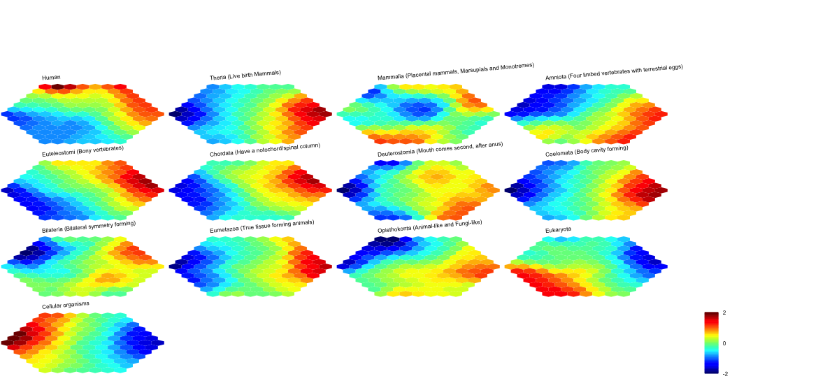
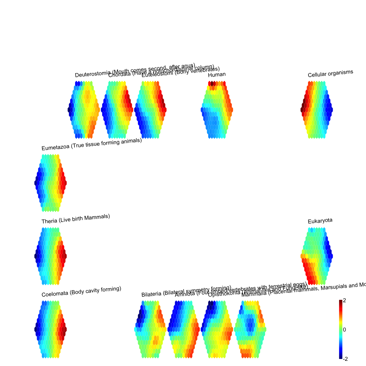
## As you have seen, a figure displays the multiple components of trained map in a sample-specific manner. You also see that a txt file
Output_Sardar_PIU.txt has been saved in your disk. The output file has 1st column for your input data ID (an integer; otherwise the row names of input data matrix), and 2nd column for the corresponding index of best-matching hexagons (i.e. cell type clusters). You can also force the input data to be output (see below).
sWriteData(sMap, data, filename="Output_Sardar_PIU_2.txt", keep.data=T)
# (III) Visualise the map, including built-in indexes, data hits/distributions, distance between map nodes, and codebook matrix
visHexMapping(sMap, mappingType="indexes")
## As you have seen, the smaller hexagons in the supra-hexagonal map are indexed as follows: start from the center, and then expand circularly outwards, and for each circle increase in an anti-clock order.
visHexMapping(sMap, mappingType="hits")
## As you have seen, the number represents how many input data vectors (cell types) are hitting each hexagon, the size of which is proportional to the number of hits.
visHexMapping(sMap, mappingType="dist")
## As you have seen, map distance tells how far each hexagon is away from its neighbors, and the size of each hexagon is proportional to this distance.
visHexPattern(sMap, plotType="lines")
## As you have seen, line plot displays the patterns associated with the codebook matrix. If multple colors are given, the points are also plotted. When the pattern involves both positive and negative values, zero horizental line is also shown.
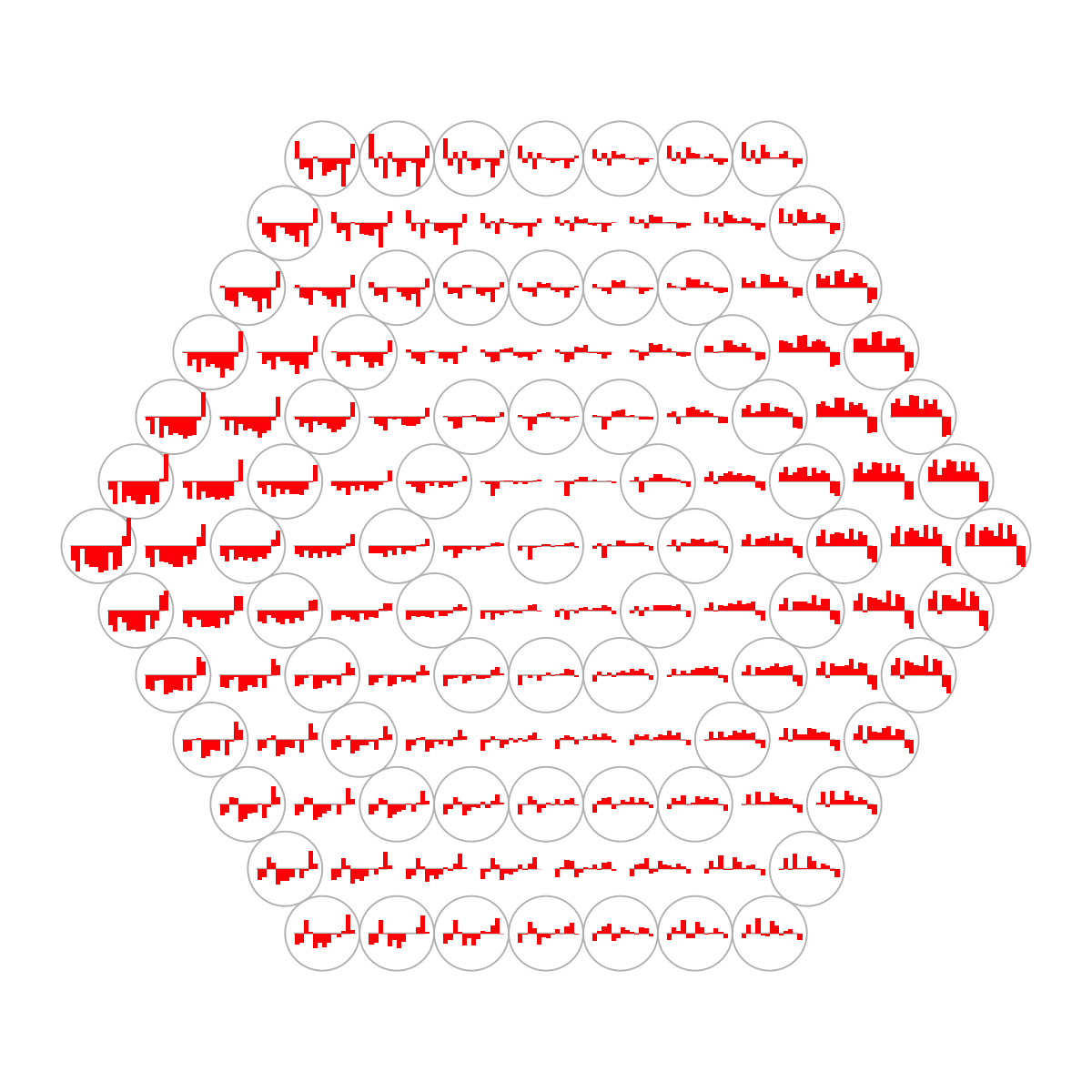
visHexPattern(sMap, plotType="bars")
## As you have seen, bar plot displays the patterns associated with the codebook matrix. When the pattern involves both positive and negative values, the zero horizental line is in the middle of the hexagon; otherwise at the top of the hexagon for all negative values, and at the bottom for all positive values.
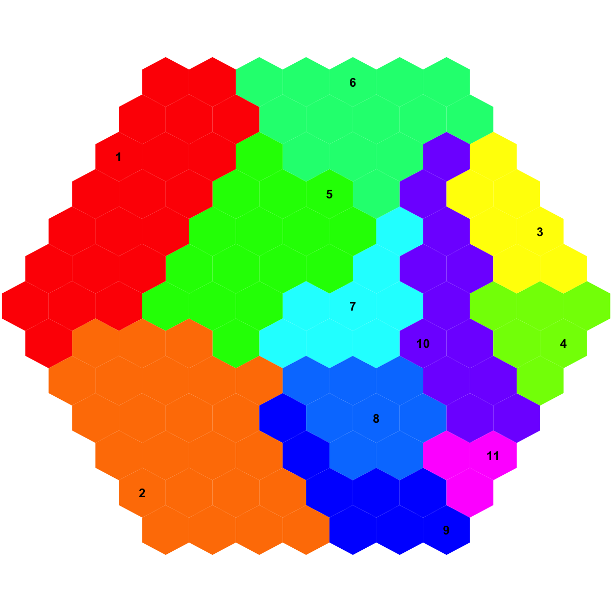
# (IV) Perform partitioning operation on the map to obtain continuous clusters (i.e. cell type meta-clusters) as they are different from cell type clusters in an individual map node
sBase <-
sDmatCluster(sMap)
 Start at 2016-06-24 11:46:28
First, define topology of a map grid (2016-06-24 11:46:28)...
Second, initialise the codebook matrix (40 X 13) using 'linear' initialisation, given a topology and input data (2016-06-24 11:46:28)...
Third, get training at the rough stage (2016-06-24 11:46:28)...
1 out of 403 (2016-06-24 11:46:28)
41 out of 403 (2016-06-24 11:46:28)
82 out of 403 (2016-06-24 11:46:28)
123 out of 403 (2016-06-24 11:46:28)
164 out of 403 (2016-06-24 11:46:28)
205 out of 403 (2016-06-24 11:46:28)
246 out of 403 (2016-06-24 11:46:28)
287 out of 403 (2016-06-24 11:46:28)
328 out of 403 (2016-06-24 11:46:28)
369 out of 403 (2016-06-24 11:46:28)
403 out of 403 (2016-06-24 11:46:28)
Fourth, get training at the finetune stage (2016-06-24 11:46:28)...
1 out of 1612 (2016-06-24 11:46:28)
162 out of 1612 (2016-06-24 11:46:28)
324 out of 1612 (2016-06-24 11:46:28)
486 out of 1612 (2016-06-24 11:46:28)
648 out of 1612 (2016-06-24 11:46:28)
810 out of 1612 (2016-06-24 11:46:29)
972 out of 1612 (2016-06-24 11:46:29)
1134 out of 1612 (2016-06-24 11:46:29)
1296 out of 1612 (2016-06-24 11:46:29)
1458 out of 1612 (2016-06-24 11:46:29)
1612 out of 1612 (2016-06-24 11:46:29)
Next, identify the best-matching hexagon/rectangle for the input data (2016-06-24 11:46:29)...
Finally, append the response data (hits and mqe) into the sMap object (2016-06-24 11:46:29)...
Below are the summaries of the training results:
dimension of input data: 13x13
xy-dimension of map grid: xdim=10, ydim=4
grid lattice: rect
grid shape: sheet
dimension of grid coord: 40x2
initialisation method: linear
dimension of codebook matrix: 40x13
mean quantization error: 23.4740407770882
Below are the details of trainology:
training algorithm: sequential
alpha type: invert
training neighborhood kernel: gaussian
trainlength (x input data length): 31 at rough stage; 124 at finetune stage
radius (at rough stage): from 2 to 1
radius (at finetune stage): from 1 to 1
End at 2016-06-24 11:46:29
Runtime in total is: 1 secs
Start at 2016-06-24 11:46:29
First, build the tree (using nj algorithm and euclidean distance) from input matrix (13 by 492)...
Second, perform bootstrap analysis with 100 replicates...
Finally, visualise the bootstrapped tree...
Start at 2016-06-24 11:46:28
First, define topology of a map grid (2016-06-24 11:46:28)...
Second, initialise the codebook matrix (40 X 13) using 'linear' initialisation, given a topology and input data (2016-06-24 11:46:28)...
Third, get training at the rough stage (2016-06-24 11:46:28)...
1 out of 403 (2016-06-24 11:46:28)
41 out of 403 (2016-06-24 11:46:28)
82 out of 403 (2016-06-24 11:46:28)
123 out of 403 (2016-06-24 11:46:28)
164 out of 403 (2016-06-24 11:46:28)
205 out of 403 (2016-06-24 11:46:28)
246 out of 403 (2016-06-24 11:46:28)
287 out of 403 (2016-06-24 11:46:28)
328 out of 403 (2016-06-24 11:46:28)
369 out of 403 (2016-06-24 11:46:28)
403 out of 403 (2016-06-24 11:46:28)
Fourth, get training at the finetune stage (2016-06-24 11:46:28)...
1 out of 1612 (2016-06-24 11:46:28)
162 out of 1612 (2016-06-24 11:46:28)
324 out of 1612 (2016-06-24 11:46:28)
486 out of 1612 (2016-06-24 11:46:28)
648 out of 1612 (2016-06-24 11:46:28)
810 out of 1612 (2016-06-24 11:46:29)
972 out of 1612 (2016-06-24 11:46:29)
1134 out of 1612 (2016-06-24 11:46:29)
1296 out of 1612 (2016-06-24 11:46:29)
1458 out of 1612 (2016-06-24 11:46:29)
1612 out of 1612 (2016-06-24 11:46:29)
Next, identify the best-matching hexagon/rectangle for the input data (2016-06-24 11:46:29)...
Finally, append the response data (hits and mqe) into the sMap object (2016-06-24 11:46:29)...
Below are the summaries of the training results:
dimension of input data: 13x13
xy-dimension of map grid: xdim=10, ydim=4
grid lattice: rect
grid shape: sheet
dimension of grid coord: 40x2
initialisation method: linear
dimension of codebook matrix: 40x13
mean quantization error: 23.4740407770882
Below are the details of trainology:
training algorithm: sequential
alpha type: invert
training neighborhood kernel: gaussian
trainlength (x input data length): 31 at rough stage; 124 at finetune stage
radius (at rough stage): from 2 to 1
radius (at finetune stage): from 1 to 1
End at 2016-06-24 11:46:29
Runtime in total is: 1 secs
Start at 2016-06-24 11:46:29
First, build the tree (using nj algorithm and euclidean distance) from input matrix (13 by 492)...
Second, perform bootstrap analysis with 100 replicates...
Finally, visualise the bootstrapped tree...
 Finish at 2016-06-24 11:46:29
Runtime in total is: 0 secs
Finish at 2016-06-24 11:46:29
Runtime in total is: 0 secs
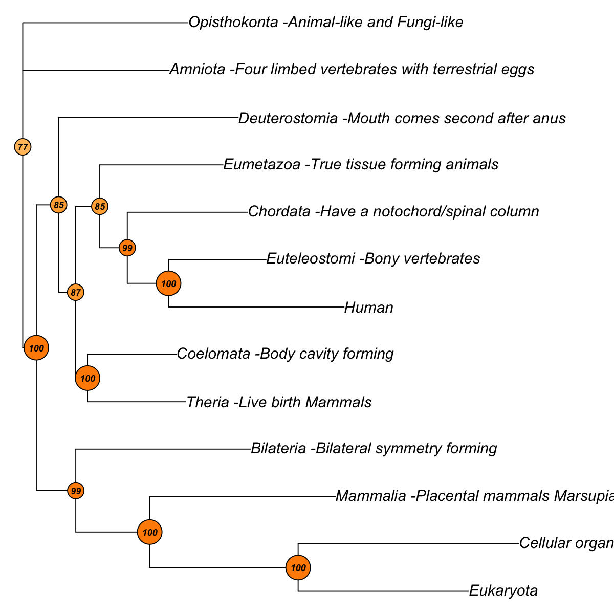
## As you have seen, neighbour-joining tree is constructed based on pairwise euclidean distance matrices between samples. The robustness of tree branching is evaluated using bootstraping. In internal nodes (also color-coded), the number represents the proportion of bootstrapped trees that support the observed internal branching. The higher the number, the more robust the tree branching. 100 means that the internal branching is always observed by resampling characters.
)
)
)
)
)
)