Loading required package: edgeR
(Intercept) celllineCellline2 celllineCellline3 treatmentDEX
1 1 0 0 0
2 1 0 0 1
3 1 1 0 0
4 1 1 0 1
5 1 0 1 0
6 1 0 1 1
attr(,"assign")
[1] 0 1 1 2
attr(,"contrasts")
attr(,"contrasts")$cellline
[1] "contr.treatment"
attr(,"contrasts")$treatment
[1] "contr.treatment"
## Inspect the relationships between samples using a multidimensional scaling (MDS) plot to show the relationship between all pairs of samples
plotMDS(d, labels=colnames(d), col=c("red","darkgreen","blue")[factor(targets$cellline)], xlim=c(-2,2), ylim=c(-2,2))

### Note: this inspection clearly shows the variances between cell lines, calling for paired design test.
# (II) Do dispersion estimation and GLM (Generalized Linear Model) fitting
# Estimate the overall dispersion to get an idea of the overall level of biological variablility
d <- estimateGLMCommonDisp(d, design, verbose=T)
Disp = 0.0048 , BCV = 0.0693
## Estimate dispersion values, relative to the design matrix, using the Cox-Reid (CR)-adjusted likelihood:
d2 <- estimateGLMTrendedDisp(d, design)
d2 <- estimateGLMTagwiseDisp(d2, design)
## Given the design matrix and dispersion estimates, fit a GLM to each feature:
f <- glmFit(d2, design)
# (III) Perform a likelihood ratio test
## Specify the difference of interest: DEX vs CON
contrasts <- rbind(c(0,0,0,1))
## Prepare the results
logFC <- matrix(nrow=nrow(d2), ncol=1)
PValue <- matrix(nrow=nrow(d2), ncol=1)
FDR <- matrix(nrow=nrow(d2), ncol=1)
tmp <- c("DEX_CON")
colnames(logFC) <- paste(tmp, '_logFC', sep='')
colnames(PValue) <- paste(tmp, '_PValue', sep='')
colnames(FDR) <- paste(tmp, '_FDR', sep='')
rownames(logFC) <- rownames(PValue) <- rownames(FDR) <- rownames(d2)
## Perform the test, calculating P-values and FDR (false discovery rate)
for(i in 1:nrow(contrasts)){
lrt <- glmLRT(f, contrast=contrasts[i,])
tt <- topTags(lrt, n=nrow(d2), adjust.method="BH", sort.by="none")
logFC[,i] <- tt$table$logFC
PValue[,i] <- tt$table$PValue
FDR[,i] <- tt$table$FDR
}
## MA plots for RNA-seq data
lrt <- glmLRT(f, contrast=contrasts[1,])
#lrt <- glmLRT(f, coef=4)
summary(de <- decideTestsDGE(lrt, adjust.method="BH", p.value=0.05))
[,1]
-1 1073
0 11311
1 1203
detags <- rownames(d2)[as.logical(de)]
plotSmear(lrt, de.tags=detags)
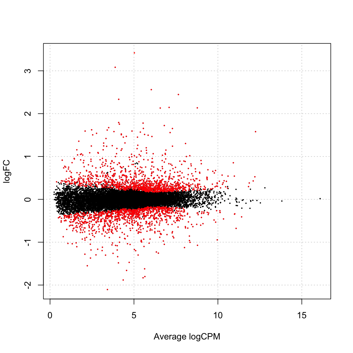
### As you have seen, it plots the log-fold change (i.e., the log ratio of normalized expression levels between two experimental conditions (i.e. DEX vs CON) against the log counts per million (CPM). Those genes selected as differentially expressed (with a 5% false discovery rate) are highlighted as red dots
# (IV) Output edgeR results
## log counts per million (CPM) for each sample
cpms <- edgeR::cpm(d2,log=T,prior.count=2)
colnames(cpms) <- paste(colnames(d2), '_CPM', sep='')
## log ratio between the treatment vs the control (for each cell line)
odd_indexes <- seq(1,ncol(cpms),2)
even_indexes <- seq(2,ncol(cpms),2)
logFC_cpm <- cpms[,even_indexes] - cpms[,odd_indexes]
colnames(logFC_cpm) <- gsub("_CPM", "_CPM_logFC", colnames(logFC_cpm), perl=T)
## write into the file 'RNAseq_edgeR.txt'
out <- data.frame(EnsemblGeneID=rownames(d2$genes), d2$genes, cpms, logFC_cpm, logFC, PValue, FDR)
write.table(out, file="RNAseq_edgeR.txt", col.names=T, row.names=F, sep="\t", quote=F)
#---------------------------------------------------------------------------
#---------------------------------------------------------------------------
# Analyse differentially expressed genes using the package 'supraHex'
#---------------------------------------------------------------------------
#---------------------------------------------------------------------------
# (I) Load the package and select differentially expressed genes identified by edgeR data
library(supraHex)
select_flag <- FDR<0.05
data <- logFC_cpm[select_flag, ]
## check the data dimension: how many genes are called significant
dim(data)
[1] 2276 3
Start at 2016-06-24 11:46:42
First, define topology of a map grid (2016-06-24 11:46:42)...
Second, initialise the codebook matrix (61 X 3) using 'linear' initialisation, given a topology and input data (2016-06-24 11:46:42)...
Third, get training at the rough stage (2016-06-24 11:46:42)...
1 out of 2276 (2016-06-24 11:46:42)
228 out of 2276 (2016-06-24 11:46:42)
456 out of 2276 (2016-06-24 11:46:42)
684 out of 2276 (2016-06-24 11:46:42)
912 out of 2276 (2016-06-24 11:46:43)
1140 out of 2276 (2016-06-24 11:46:43)
1368 out of 2276 (2016-06-24 11:46:43)
1596 out of 2276 (2016-06-24 11:46:43)
1824 out of 2276 (2016-06-24 11:46:43)
2052 out of 2276 (2016-06-24 11:46:43)
2276 out of 2276 (2016-06-24 11:46:43)
Fourth, get training at the finetune stage (2016-06-24 11:46:43)...
1 out of 4552 (2016-06-24 11:46:43)
456 out of 4552 (2016-06-24 11:46:43)
912 out of 4552 (2016-06-24 11:46:43)
1368 out of 4552 (2016-06-24 11:46:43)
1824 out of 4552 (2016-06-24 11:46:43)
2280 out of 4552 (2016-06-24 11:46:43)
2736 out of 4552 (2016-06-24 11:46:43)
3192 out of 4552 (2016-06-24 11:46:44)
3648 out of 4552 (2016-06-24 11:46:44)
4104 out of 4552 (2016-06-24 11:46:44)
4552 out of 4552 (2016-06-24 11:46:44)
Next, identify the best-matching hexagon/rectangle for the input data (2016-06-24 11:46:44)...
Finally, append the response data (hits and mqe) into the sMap object (2016-06-24 11:46:44)...
Below are the summaries of the training results:
dimension of input data: 2276x3
xy-dimension of map grid: xdim=9, ydim=9
grid lattice: hexa
grid shape: suprahex
dimension of grid coord: 61x2
initialisation method: linear
dimension of codebook matrix: 61x3
mean quantization error: 0.148236509445458
Below are the details of trainology:
training algorithm: sequential
alpha type: invert
training neighborhood kernel: gaussian
trainlength (x input data length): 1 at rough stage; 2 at finetune stage
radius (at rough stage): from 3 to 1
radius (at finetune stage): from 1 to 1
End at 2016-06-24 11:46:44
Runtime in total is: 2 secs
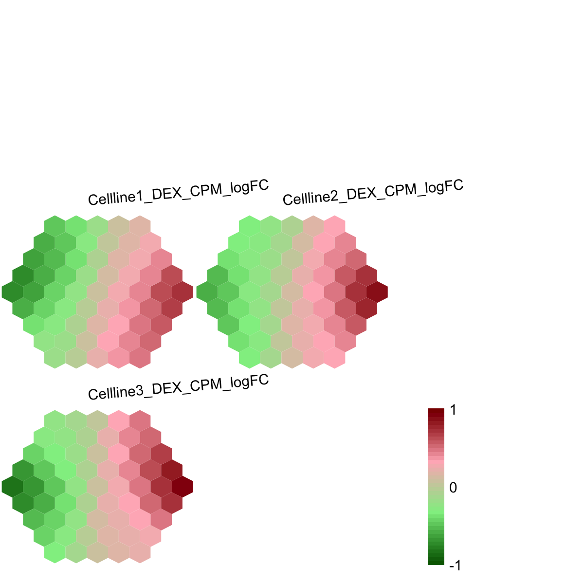
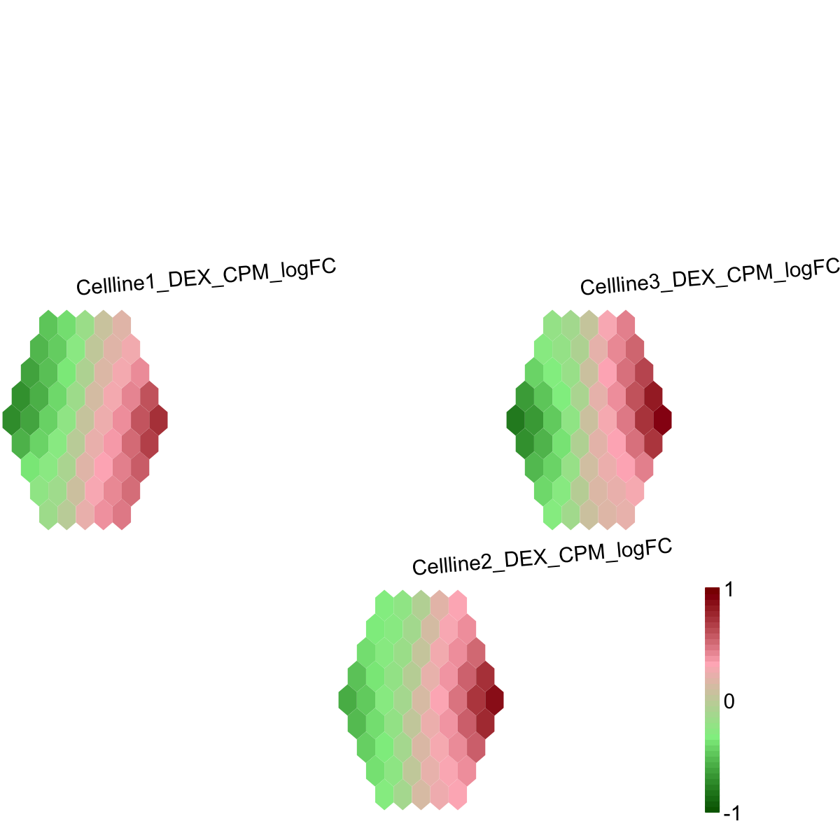
## As you have seen, a figure displays the multiple components of trained map in a sample-specific manner. You also see that a txt file
RNAseq_edgeR.supraHex.txt has been saved in your disk. The output file has 1st column for your input data ID (an integer; otherwise the row names of input data matrix), and 2nd column for the corresponding index of best-matching hexagons (i.e. gene clusters). You can also force the input data to be output (see below).
sWriteData(sMap, data, filename="RNAseq_edgeR.supraHex_2.txt", keep.data=T)
# (III) Visualise the map, including built-in indexes, data hits/distributions, distance between map nodes, and codebook matrix
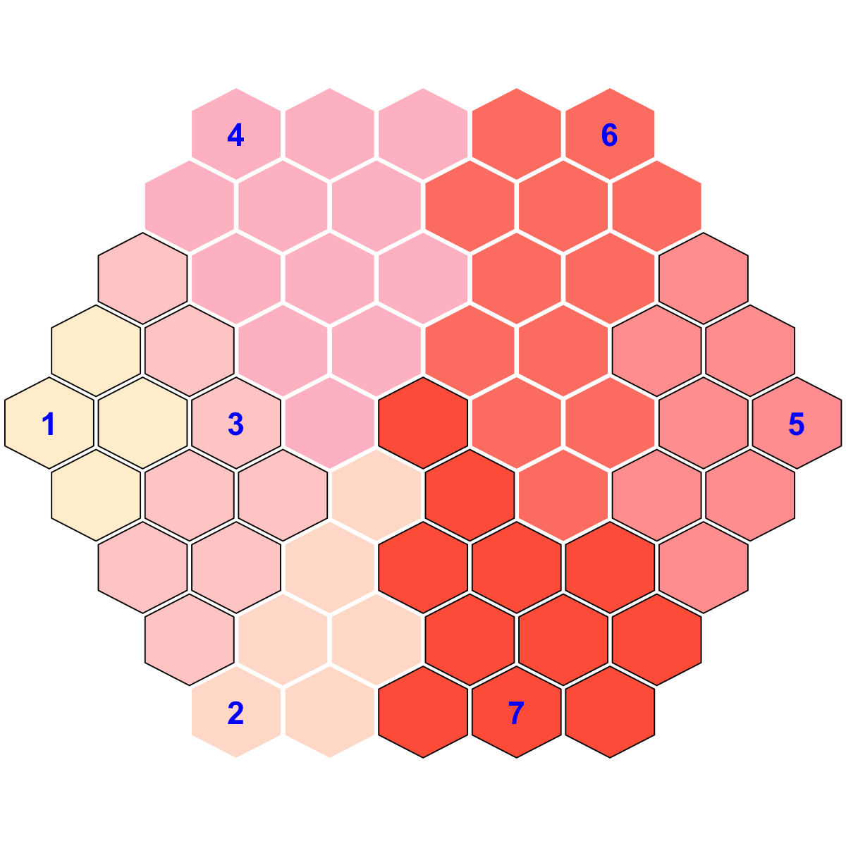
visHexMapping(sMap, mappingType="indexes")
## As you have seen, the smaller hexagons in the supra-hexagonal map are indexed as follows: start from the center, and then expand circularly outwards, and for each circle increase in an anti-clock order.
visHexMapping(sMap, mappingType="hits")
## As you have seen, the number represents how many input data vectors (mutations) are hitting each hexagon, the size of which is proportional to the number of hits.
visHexMapping(sMap, mappingType="dist")
## As you have seen, map distance tells how far each hexagon is away from its neighbors, and the size of each hexagon is proportional to this distance.
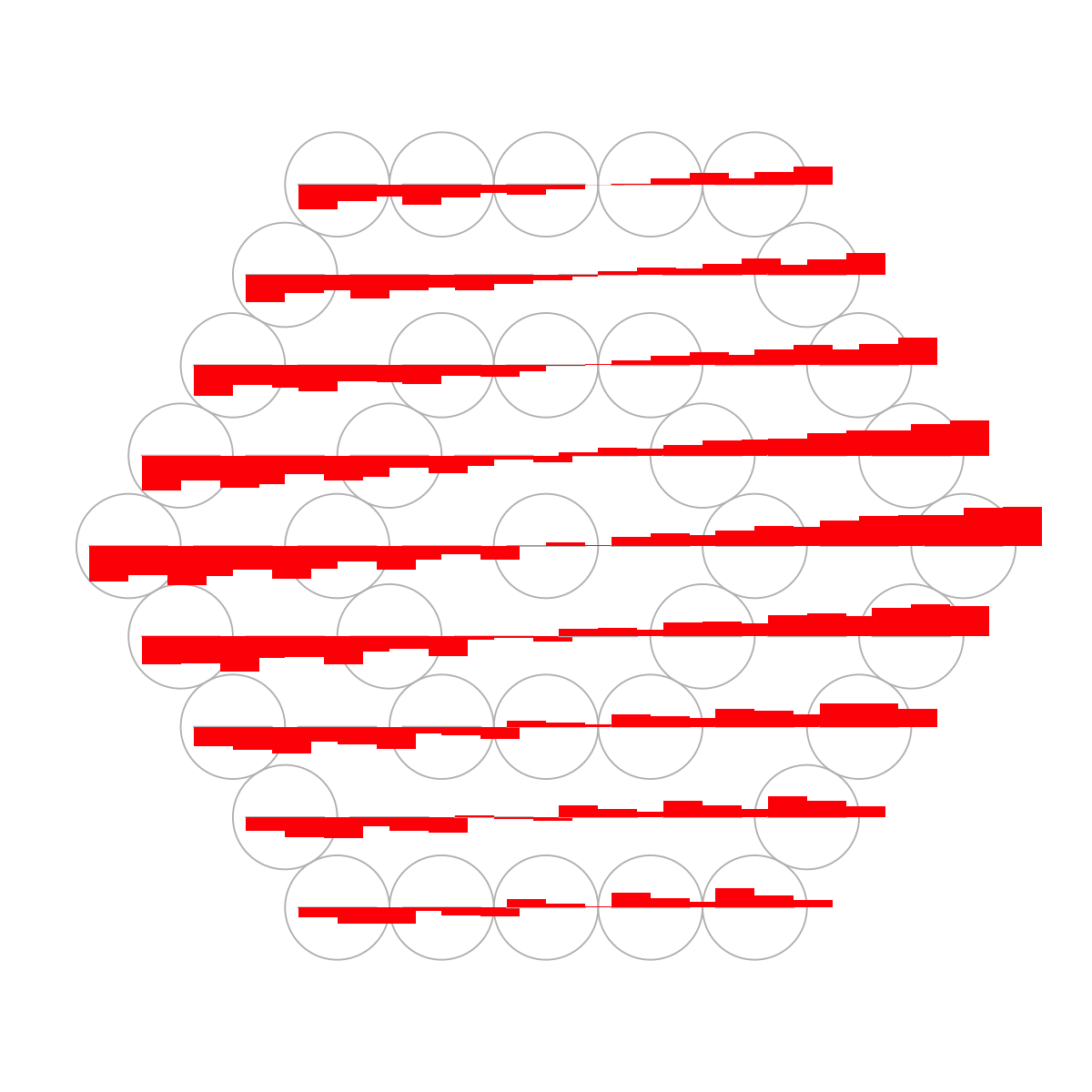
visHexPattern(sMap, plotType="lines")
## As you have seen, line plot displays the patterns associated with the codebook matrix. If multple colors are given, the points are also plotted. When the pattern involves both positive and negative values, zero horizental line is also shown.
visHexPattern(sMap, plotType="bars")
## As you have seen, bar plot displays the patterns associated with the codebook matrix. When the pattern involves both positive and negative values, the zero horizental line is in the middle of the hexagon; otherwise at the top of the hexagon for all negative values, and at the bottom for all positive values.
# (IV) Perform partitioning operation on the map to obtain continuous clusters (i.e. gene meta-clusters) as they are different from gene clusters in an individual map node
sBase <-
sDmatCluster(sMap)
 Start at 2016-06-24 11:46:45
First, define topology of a map grid (2016-06-24 11:46:45)...
Second, initialise the codebook matrix (8 X 3) using 'linear' initialisation, given a topology and input data (2016-06-24 11:46:45)...
Third, get training at the rough stage (2016-06-24 11:46:45)...
1 out of 81 (2016-06-24 11:46:45)
9 out of 81 (2016-06-24 11:46:45)
18 out of 81 (2016-06-24 11:46:45)
27 out of 81 (2016-06-24 11:46:45)
36 out of 81 (2016-06-24 11:46:45)
45 out of 81 (2016-06-24 11:46:45)
54 out of 81 (2016-06-24 11:46:45)
63 out of 81 (2016-06-24 11:46:45)
72 out of 81 (2016-06-24 11:46:45)
81 out of 81 (2016-06-24 11:46:45)
Fourth, get training at the finetune stage (2016-06-24 11:46:45)...
1 out of 321 (2016-06-24 11:46:45)
33 out of 321 (2016-06-24 11:46:45)
66 out of 321 (2016-06-24 11:46:45)
99 out of 321 (2016-06-24 11:46:45)
132 out of 321 (2016-06-24 11:46:45)
165 out of 321 (2016-06-24 11:46:45)
198 out of 321 (2016-06-24 11:46:45)
231 out of 321 (2016-06-24 11:46:45)
264 out of 321 (2016-06-24 11:46:45)
297 out of 321 (2016-06-24 11:46:45)
321 out of 321 (2016-06-24 11:46:45)
Next, identify the best-matching hexagon/rectangle for the input data (2016-06-24 11:46:45)...
Finally, append the response data (hits and mqe) into the sMap object (2016-06-24 11:46:45)...
Below are the summaries of the training results:
dimension of input data: 3x3
xy-dimension of map grid: xdim=4, ydim=2
grid lattice: rect
grid shape: sheet
dimension of grid coord: 8x2
initialisation method: linear
dimension of codebook matrix: 8x3
mean quantization error: 0.0386044771959701
Below are the details of trainology:
training algorithm: sequential
alpha type: invert
training neighborhood kernel: gaussian
trainlength (x input data length): 27 at rough stage; 107 at finetune stage
radius (at rough stage): from 1 to 1
radius (at finetune stage): from 1 to 1
End at 2016-06-24 11:46:45
Runtime in total is: 0 secs
Start at 2016-06-24 11:46:45
First, define topology of a map grid (2016-06-24 11:46:45)...
Second, initialise the codebook matrix (8 X 3) using 'linear' initialisation, given a topology and input data (2016-06-24 11:46:45)...
Third, get training at the rough stage (2016-06-24 11:46:45)...
1 out of 81 (2016-06-24 11:46:45)
9 out of 81 (2016-06-24 11:46:45)
18 out of 81 (2016-06-24 11:46:45)
27 out of 81 (2016-06-24 11:46:45)
36 out of 81 (2016-06-24 11:46:45)
45 out of 81 (2016-06-24 11:46:45)
54 out of 81 (2016-06-24 11:46:45)
63 out of 81 (2016-06-24 11:46:45)
72 out of 81 (2016-06-24 11:46:45)
81 out of 81 (2016-06-24 11:46:45)
Fourth, get training at the finetune stage (2016-06-24 11:46:45)...
1 out of 321 (2016-06-24 11:46:45)
33 out of 321 (2016-06-24 11:46:45)
66 out of 321 (2016-06-24 11:46:45)
99 out of 321 (2016-06-24 11:46:45)
132 out of 321 (2016-06-24 11:46:45)
165 out of 321 (2016-06-24 11:46:45)
198 out of 321 (2016-06-24 11:46:45)
231 out of 321 (2016-06-24 11:46:45)
264 out of 321 (2016-06-24 11:46:45)
297 out of 321 (2016-06-24 11:46:45)
321 out of 321 (2016-06-24 11:46:45)
Next, identify the best-matching hexagon/rectangle for the input data (2016-06-24 11:46:45)...
Finally, append the response data (hits and mqe) into the sMap object (2016-06-24 11:46:45)...
Below are the summaries of the training results:
dimension of input data: 3x3
xy-dimension of map grid: xdim=4, ydim=2
grid lattice: rect
grid shape: sheet
dimension of grid coord: 8x2
initialisation method: linear
dimension of codebook matrix: 8x3
mean quantization error: 0.0386044771959701
Below are the details of trainology:
training algorithm: sequential
alpha type: invert
training neighborhood kernel: gaussian
trainlength (x input data length): 27 at rough stage; 107 at finetune stage
radius (at rough stage): from 1 to 1
radius (at finetune stage): from 1 to 1
End at 2016-06-24 11:46:45
Runtime in total is: 0 secs
)
)
)
)
)
)
)