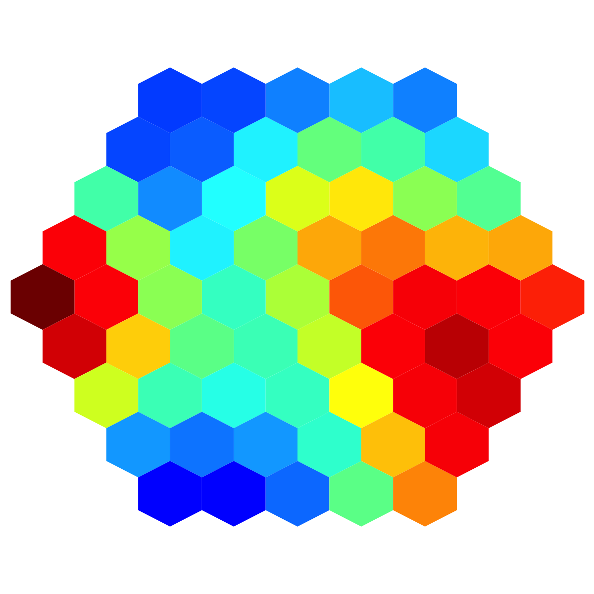
Function to visualise a component plane of a supra-hexagonal grid
Description
visHexComp is supposed to visualise a supra-hexagonal grid in
the context of viewport
Usage
visHexComp(sMap, comp, margin = rep(0.6, 4), area.size = 1, colormap = c("bwr", "jet",
  "gbr", "wyr", "br", "yr", "rainbow", "wb"), ncolors = 40, zlim = c(0, 1), border.color = "transparent",
      newpage = TRUE)
Arguments
- sMap
- an object of class "sMap"
- comp
- a component/column of codebook matrix from an object "sMap"
- margin
- margins as units of length 4 or 1
- area.size
- an inteter or a vector specifying the area size of each hexagon
- colormap
- short name for the colormap. It can be one of "jet" (jet colormap), "bwr" (blue-white-red colormap), "gbr" (green-black-red colormap), "wyr" (white-yellow-red colormap), "br" (black-red colormap), "yr" (yellow-red colormap), "wb" (white-black colormap), and "rainbow" (rainbow colormap, that is, red-yellow-green-cyan-blue-magenta). Alternatively, any hyphen-separated HTML color names, e.g. "blue-black-yellow", "royalblue-white-sandybrown", "darkgreen-white-darkviolet". A list of standard color names can be found in http://html-color-codes.info/color-names
- ncolors
- the number of colors specified
- zlim
- the minimum and maximum z values for which colors should be plotted, defaulting to the range of the finite values of z. Each of the given colors will be used to color an equispaced interval of this range. The midpoints of the intervals cover the range, so that values just outside the range will be plotted
- border.color
- the border color for each hexagon
- newpage
- a logical to indicate whether or not to open a new page
Value
invisible
Note
none
Examples
# 1) generate an iid normal random matrix of 100x10 data <- matrix( rnorm(100*10,mean=0,sd=1), nrow=100, ncol=10) colnames(data) <- paste(rep('S',10), seq(1:10), sep="") # 2) sMap resulted from using by default setup sMap <- sPipeline(data=data)Start at 2018-01-18 16:56:27 First, define topology of a map grid (2018-01-18 16:56:27)... Second, initialise the codebook matrix (61 X 10) using 'linear' initialisation, given a topology and input data (2018-01-18 16:56:27)... Third, get training at the rough stage (2018-01-18 16:56:27)... 1 out of 7 (2018-01-18 16:56:27) updated (2018-01-18 16:56:27) 2 out of 7 (2018-01-18 16:56:27) updated (2018-01-18 16:56:27) 3 out of 7 (2018-01-18 16:56:27) updated (2018-01-18 16:56:27) 4 out of 7 (2018-01-18 16:56:27) updated (2018-01-18 16:56:27) 5 out of 7 (2018-01-18 16:56:27) updated (2018-01-18 16:56:27) 6 out of 7 (2018-01-18 16:56:27) updated (2018-01-18 16:56:27) 7 out of 7 (2018-01-18 16:56:27) updated (2018-01-18 16:56:27) Fourth, get training at the finetune stage (2018-01-18 16:56:27)... 1 out of 25 (2018-01-18 16:56:27) updated (2018-01-18 16:56:27) 2 out of 25 (2018-01-18 16:56:27) updated (2018-01-18 16:56:27) 3 out of 25 (2018-01-18 16:56:27) updated (2018-01-18 16:56:27) 4 out of 25 (2018-01-18 16:56:27) updated (2018-01-18 16:56:27) 5 out of 25 (2018-01-18 16:56:27) updated (2018-01-18 16:56:27) 6 out of 25 (2018-01-18 16:56:27) updated (2018-01-18 16:56:27) 7 out of 25 (2018-01-18 16:56:27) updated (2018-01-18 16:56:27) 8 out of 25 (2018-01-18 16:56:27) updated (2018-01-18 16:56:27) 9 out of 25 (2018-01-18 16:56:27) updated (2018-01-18 16:56:27) 10 out of 25 (2018-01-18 16:56:27) updated (2018-01-18 16:56:27) 11 out of 25 (2018-01-18 16:56:27) updated (2018-01-18 16:56:27) 12 out of 25 (2018-01-18 16:56:27) updated (2018-01-18 16:56:27) 13 out of 25 (2018-01-18 16:56:27) updated (2018-01-18 16:56:27) 14 out of 25 (2018-01-18 16:56:27) updated (2018-01-18 16:56:27) 15 out of 25 (2018-01-18 16:56:27) updated (2018-01-18 16:56:27) 16 out of 25 (2018-01-18 16:56:27) updated (2018-01-18 16:56:27) 17 out of 25 (2018-01-18 16:56:27) updated (2018-01-18 16:56:27) 18 out of 25 (2018-01-18 16:56:27) updated (2018-01-18 16:56:27) 19 out of 25 (2018-01-18 16:56:27) updated (2018-01-18 16:56:27) 20 out of 25 (2018-01-18 16:56:27) updated (2018-01-18 16:56:27) 21 out of 25 (2018-01-18 16:56:27) updated (2018-01-18 16:56:27) 22 out of 25 (2018-01-18 16:56:27) updated (2018-01-18 16:56:27) 23 out of 25 (2018-01-18 16:56:27) updated (2018-01-18 16:56:27) 24 out of 25 (2018-01-18 16:56:27) updated (2018-01-18 16:56:27) 25 out of 25 (2018-01-18 16:56:27) updated (2018-01-18 16:56:27) Next, identify the best-matching hexagon/rectangle for the input data (2018-01-18 16:56:27)... Finally, append the response data (hits and mqe) into the sMap object (2018-01-18 16:56:27)... Below are the summaries of the training results: dimension of input data: 100x10 xy-dimension of map grid: xdim=9, ydim=9, r=5 grid lattice: hexa grid shape: suprahex dimension of grid coord: 61x2 initialisation method: linear dimension of codebook matrix: 61x10 mean quantization error: 4.9630432442287 Below are the details of trainology: training algorithm: batch alpha type: invert training neighborhood kernel: gaussian trainlength (x input data length): 7 at rough stage; 25 at finetune stage radius (at rough stage): from 3 to 1 radius (at finetune stage): from 1 to 1 End at 2018-01-18 16:56:27 Runtime in total is: 0 secs# 3) visualise the first component plane with a supra-hexagonal grid visHexComp(sMap, comp=sMap$codebook[,1], colormap="jet", ncolors=100, zlim=c(-1,1))
