# This is a demo for the artwork in ISMB 2014
# 
# This artwork is produced using the human embryo expression dataset (available from http://www.ncbi.nlm.nih.gov/pubmed/20643359) involves six successive developmental stages (S9-S14) with three replicates (R1-R3) for each stage, including:
## Fang: an expression matrix of 5,441 genes X 18 samples;
## Fang.geneinfo: a matrix of 5,441 X 3 containing gene information;
## Fang.sampleinfo: a matrix of 18 X 3 containing sample information.
###############################################################################

# Load the package 'supraHex'
library(supraHex)

# Load and/or install packages used in this demo
for(pkg in c("Biobase","limma")){
    if(!require(pkg, character.only=T)){
        source("http://bioconductor.org/biocLite.R")
        biocLite(pkg)
        lapply(pkg, library, character.only=T)
    }
}

Loading required package: Biobase
Loading required package: BiocGenerics
Loading required package: parallel

Attaching package: ‘BiocGenerics’

The following objects are masked from ‘package:parallel’:

    clusterApply, clusterApplyLB, clusterCall, clusterEvalQ,
    clusterExport, clusterMap, parApply, parCapply, parLapply,
    parLapplyLB, parRapply, parSapply, parSapplyLB

The following object is masked from ‘package:stats’:

    xtabs

The following objects are masked from ‘package:base’:

    anyDuplicated, append, as.data.frame, as.vector, cbind, colnames,
    do.call, duplicated, eval, evalq, Filter, Find, get, intersect,
    is.unsorted, lapply, Map, mapply, match, mget, order, paste, pmax,
    pmax.int, pmin, pmin.int, Position, rank, rbind, Reduce, rep.int,
    rownames, sapply, setdiff, sort, table, tapply, union, unique,
    unlist, unsplit

Welcome to Bioconductor

    Vignettes contain introductory material; view with
    'browseVignettes()'. To cite Bioconductor, see
    'citation("Biobase")', and for packages 'citation("pkgname")'.

Loading required package: limma

Attaching package: ‘limma’

The following object is masked from ‘package:BiocGenerics’:

    plotMA


############################################################
# Preprocess data (this should be done as your data suggest)
############################################################

# import data containing three variables ('Fang', 'Fang.geneinfo' and 'Fang.sampleinfo')
data(Fang)
data <- Fang
fdata <- as.data.frame(Fang.geneinfo[,2:3])
rownames(fdata) <- Fang.geneinfo[,1]
pdata <- as.data.frame(Fang.sampleinfo[,2:3])
rownames(pdata) <- Fang.sampleinfo[,1]

# create the 'eset' object
colmatch <- match(rownames(pdata),colnames(data))
rowmatch <- match(rownames(fdata),rownames(data))
data <- data[rowmatch,colmatch]
eset <- new("ExpressionSet", exprs=as.matrix(data), phenoData=as(pdata,"AnnotatedDataFrame"), featureData=as(fdata,"AnnotatedDataFrame"))

# A function to convert probeset-centric to entrezgene-centric expression levels
prob2gene <- function(eset){
    fdat <- fData(eset)
    tmp <- as.matrix(unique(fdat[c("EntrezGene", "Symbol")]))
    forder <- tmp[order(as.numeric(tmp[,1])),]
    forder <- forder[!is.na(forder[,1]),]
    rownames(forder) <- forder[,2]
    system.time({
        dat <- exprs(eset)
        edat <- matrix(data=NA, nrow=nrow(forder), ncol=ncol(dat))
        for (i in 1:nrow(forder)){
            ind <- which(fdat$EntrezGene==as.numeric(forder[i,1]))
            if (length(ind) == 1){
                edat[i,] <- dat[ind,]
            }else{
                edat[i,] <- apply(dat[ind,],2,mean)
            }
        }
    })
    
    rownames(edat) <- rownames(forder) # as gene symbols
    colnames(edat) <- rownames(pData(eset))
    esetGene <- new('ExpressionSet',exprs=data.frame(edat),phenoData=as(pData(eset),"AnnotatedDataFrame"),featureData=as(data.frame(forder),"AnnotatedDataFrame"))
    return(esetGene)
}
esetGene <- prob2gene(eset)
esetGene

ExpressionSet (storageMode: lockedEnvironment)
assayData: 4139 features, 18 samples 
  element names: exprs 
protocolData: none
phenoData
  sampleNames: S9_R1 S9_R2 ... S14_R3 (18 total)
  varLabels: Stage Replicate
  varMetadata: labelDescription
featureData
  featureNames: A2M AADAC ... LOC100131613 (4139 total)
  fvarLabels: EntrezGene Symbol
  fvarMetadata: labelDescription
experimentData: use 'experimentData(object)'
Annotation:  


# prepare the expression matrix: relative to mean expression level across stages
D <- as.matrix(exprs(esetGene))
D <- D - as.matrix(apply(D,1,mean),ncol=1)[,rep(1,ncol(D))]

# only focus on differentially expressed genes
library(dnet)

Loading required package: igraph

Attaching package: ‘igraph’

The following objects are masked from ‘package:BiocGenerics’:

    normalize, union

The following object is masked from ‘package:testthat’:

    compare

The following object is masked from ‘package:stringr’:

    %>%

The following objects are masked from ‘package:stats’:

    decompose, spectrum

The following object is masked from ‘package:base’:

    union

Error: package ‘supraHex’ required by ‘dnet’ could not be found
## define the design matrix in a order manner
all <- as.vector(pData(esetGene)$Stage)
level <- levels(factor(all))
index_level <- sapply(level, function(x) which(all==x)[1])
level_sorted <- all[sort(index_level, decreasing=F)]
design <- sapply(level_sorted, function(x) as.numeric(all==x)) # Convert a factor column to multiple boolean columns
## a linear model is fitted for every gene by the function lmFit
fit <- lmFit(exprs(esetGene), design)
## define a contrast matrix
### contrast against the average
tmp_all <- paste(level_sorted, collapse="+")
tmp_ave <- paste("(",tmp_all,")/",length(level_sorted), sep="")
tmp_each <- sapply(level_sorted, function(x){
	paste(x,"-",tmp_ave, sep="")
})
name_contrast <- sapply(level_sorted, function(x){
	paste(x, sep="")
})
contrasts <- list(each = tmp_each,name = name_contrast)
contrast.matrix <- makeContrasts(contrasts=contrasts$each, levels=design)
colnames(contrast.matrix) <- contrasts$name
## computes moderated t-statistics and log-odds of differential expression by empirical Bayes shrinkage of the standard errors towards a common value
fit2 <- contrasts.fit(fit, contrast.matrix)
fit2 <- eBayes(fit2)
## for p-value
pvals <- as.matrix(fit2$p.value)
## for adjusted p-value
adjpvals <- sapply(1:ncol(pvals),function(x) {
    p.adjust(pvals[,x], method="BH")
})
colnames(adjpvals) <- colnames(pvals)
## select differentially expressed genes
flag <- apply(adjpvals<1e-2, 1, sum)
data <- as.matrix(fit2$coefficients[flag>=1,])

############################################################
# Now analyse 'data' prepared above by the package 'supraHex'
############################################################
# (I) Train the supra-hexagonal map with input data only
sMap <- sPipeline(data, xdim=13)

Start at 2016-06-24 11:46:25

First, define topology of a map grid (2016-06-24 11:46:25)...
Second, initialise the codebook matrix (127 X 6) using 'linear' initialisation, given a topology and input data (2016-06-24 11:46:25)...
Third, get training at the rough stage (2016-06-24 11:46:25)...
	1 out of 2 (2016-06-24 11:46:25)
	updated (2016-06-24 11:46:25)
	2 out of 2 (2016-06-24 11:46:25)
	updated (2016-06-24 11:46:25)
Fourth, get training at the finetune stage (2016-06-24 11:46:25)...
	1 out of 2 (2016-06-24 11:46:25)
	updated (2016-06-24 11:46:25)
	2 out of 2 (2016-06-24 11:46:25)
	updated (2016-06-24 11:46:25)
Next, identify the best-matching hexagon/rectangle for the input data (2016-06-24 11:46:25)...
Finally, append the response data (hits and mqe) into the sMap object (2016-06-24 11:46:26)...

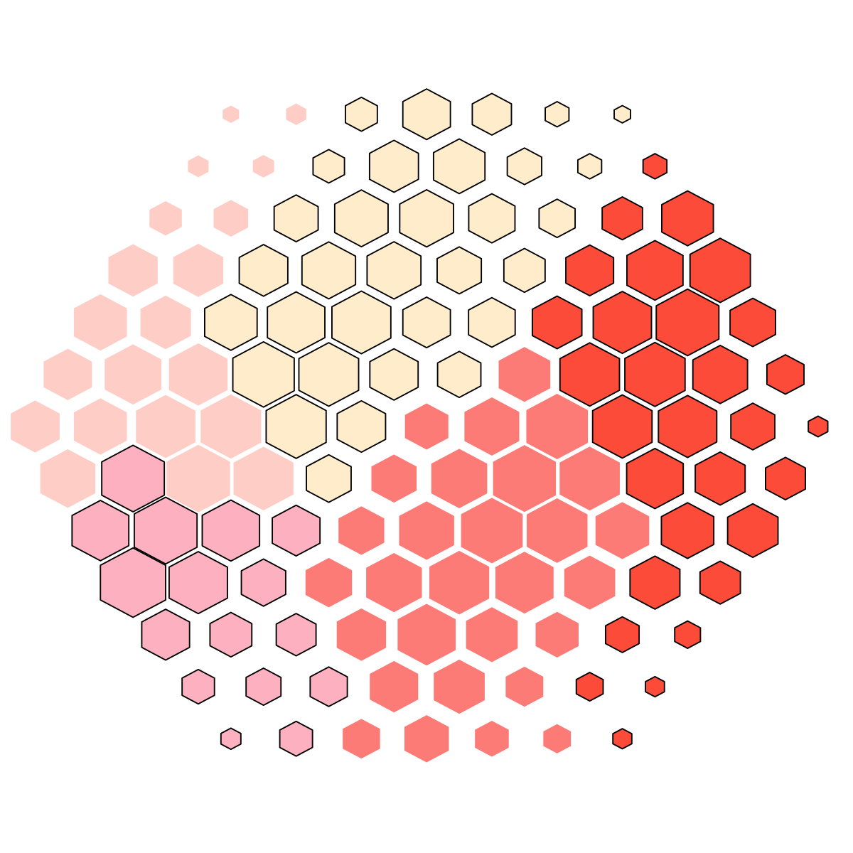
Below are the summaries of the training results:
   dimension of input data: 4018x6
   xy-dimension of map grid: xdim=13, ydim=13
   grid lattice: hexa
   grid shape: suprahex
   dimension of grid coord: 127x2
   initialisation method: linear
   dimension of codebook matrix: 127x6
   mean quantization error: 0.108267518704114

Below are the details of trainology:
   training algorithm: batch
   alpha type: invert
   training neighborhood kernel: gaussian
   trainlength (x input data length): 2 at rough stage; 2 at finetune stage
   radius (at rough stage): from 4 to 1
   radius (at finetune stage): from 1 to 1

End at 2016-06-24 11:46:26
Runtime in total is: 1 secs


# (II) Perform partitioning operation on the map to obtain continuous clusters (i.e. gene meta-clusters) as they are different from gene clusters in an individual map node
sBase <- sDmatCluster(sMap, which_neigh=2, reindexSeed="svd")

# (III) Define visuals
## the hexagon frame according to mete-clusters
myColor <- c("transparent", "black")
border.color <- myColor[sBase$bases%%2 + 1]
## the size of hexagon according to distance to their neighours
dMat <- sDmat(sMap, which_neigh = 2, distMeasure = "median")

# (IV) Do visualisation in a single map
visDmatCluster(sMap,sBase, gp=grid::gpar(cex=1.5, font=2, col="transparent"), colormap="PapayaWhip-pink-Tomato", area.size=-1*log2(dMat), border.color=border.color)
# As you have seen, the map distance (the hexagon size) tells how far each node is away from its neighbors, thus characterising relationships between clustered genes. The map is also partitioned to obtain gene meta-clusters covering continuous regions, as colour-coded by the 'potato-peach-tomato' colormap.

      

Source demo

Functions used in this demo

• sPipeline
• sDmatCluster
• sDmat
• visDmatCluster