[1] "CpG" "EX" "RT" "URL"
Start at 2016-06-24 11:44:36
First, define topology of a map grid (2016-06-24 11:44:36)...
Second, initialise the codebook matrix (721 X 22) using 'linear' initialisation, given a topology and input data (2016-06-24 11:44:36)...
Third, get training at the rough stage (2016-06-24 11:44:36)...
1 out of 2 (2016-06-24 11:44:36)
updated (2016-06-24 11:44:38)
2 out of 2 (2016-06-24 11:44:38)
updated (2016-06-24 11:44:40)
Fourth, get training at the finetune stage (2016-06-24 11:44:40)...
1 out of 2 (2016-06-24 11:44:40)
updated (2016-06-24 11:44:42)
2 out of 2 (2016-06-24 11:44:42)
updated (2016-06-24 11:44:44)
Next, identify the best-matching hexagon/rectangle for the input data (2016-06-24 11:44:44)...
Finally, append the response data (hits and mqe) into the sMap object (2016-06-24 11:44:46)...
Below are the summaries of the training results:
dimension of input data: 17292x22
xy-dimension of map grid: xdim=31, ydim=31
grid lattice: hexa
grid shape: suprahex
dimension of grid coord: 721x2
initialisation method: linear
dimension of codebook matrix: 721x22
mean quantization error: 1.72760785618509
Below are the details of trainology:
training algorithm: batch
alpha type: invert
training neighborhood kernel: gaussian
trainlength (x input data length): 2 at rough stage; 2 at finetune stage
radius (at rough stage): from 8 to 2
radius (at finetune stage): from 2 to 1
End at 2016-06-24 11:44:46
Runtime in total is: 10 secs
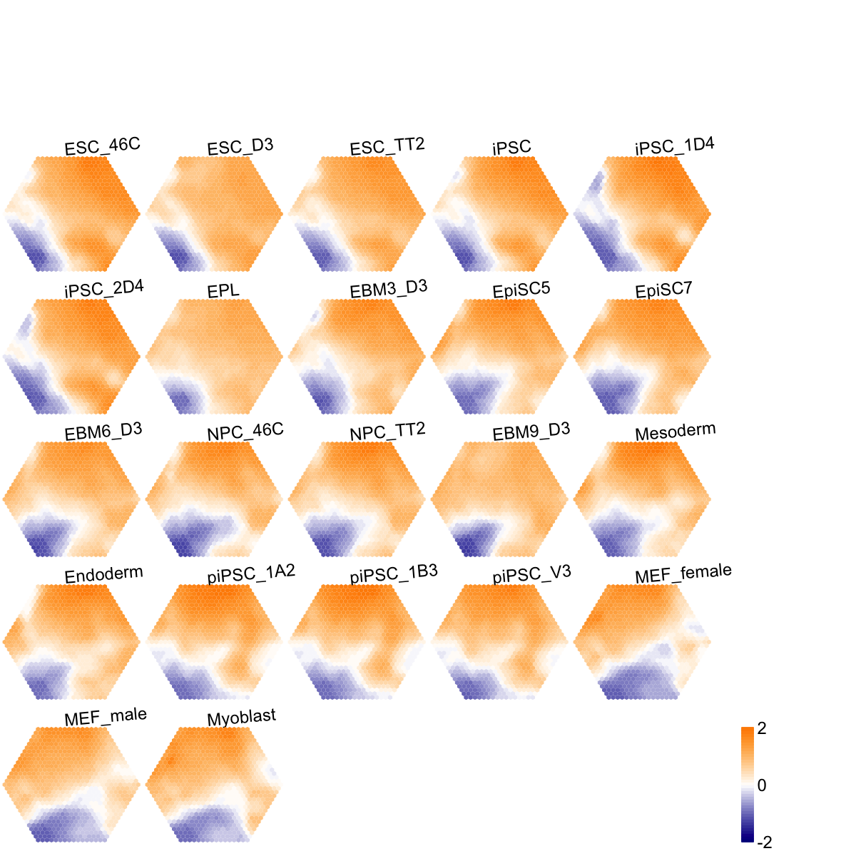
## As you have seen, a figure displays the multiple components of trained map in a sample-specific manner. You also see that a .txt file has been saved in your disk. The output file has 1st column for your input data ID (an integer; otherwise the row names of input data matrix), and 2nd column for the corresponding index of best-matching hexagons (i.e. gene clusters). You can also force the input data to be output; type ?
sWriteData for details.
# (III) Visualise the map, including built-in indexes, data hits/distributions, distance between map nodes, and codebook matrix
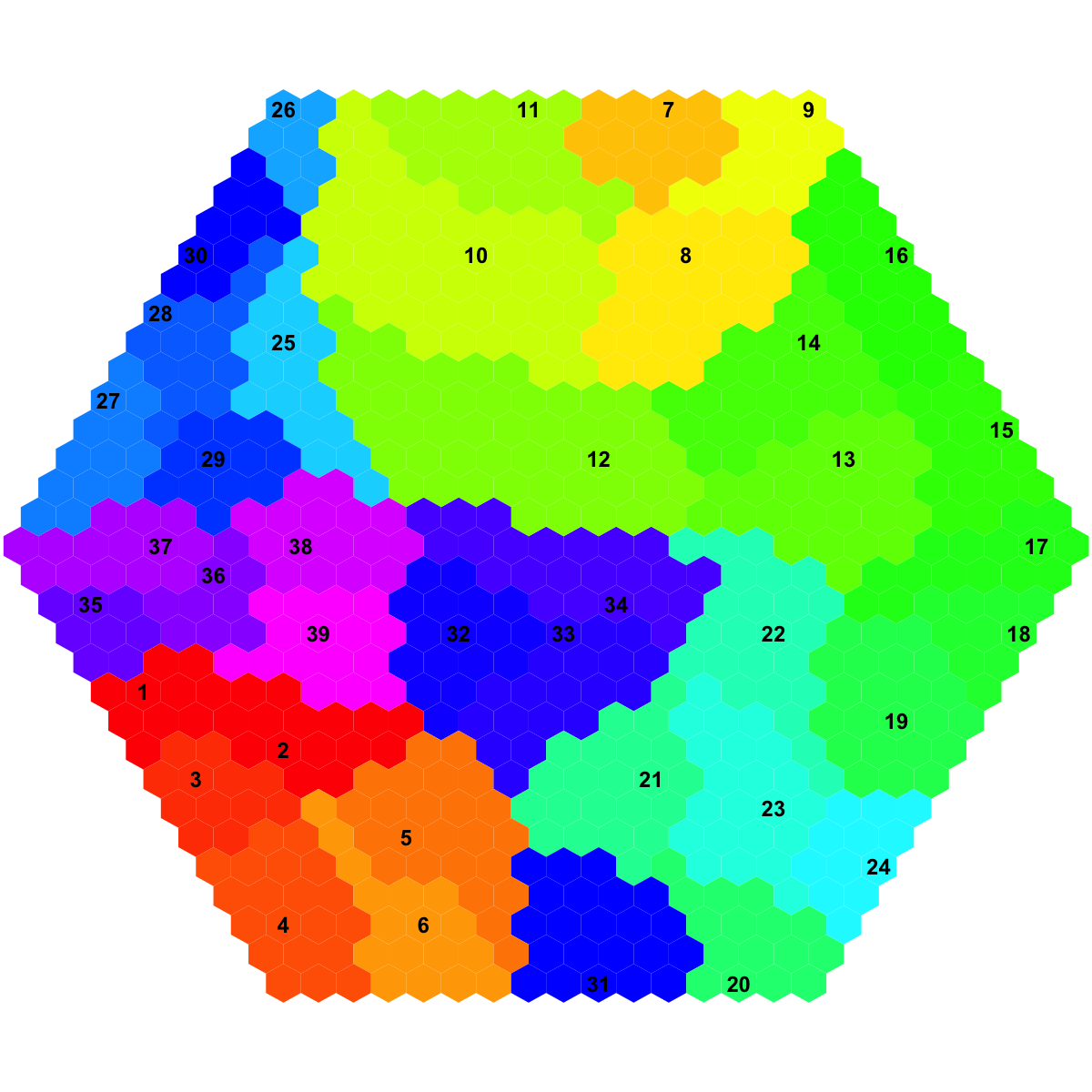
visHexMapping(sMap, mappingType="indexes", gp=grid::gpar(cex=0.5))
## As you have seen, the smaller hexagons in the supra-hexagonal map are indexed as follows: start from the center, and then expand circularly outwards, and for each circle increase in an anti-clock order.
visHexMapping(sMap, mappingType="hits", gp=grid::gpar(cex=0.5))
## As you have seen, the number represents how many input data vectors are hitting each hexagon, the size of which is proportional to the number of hits.
visHexMapping(sMap, mappingType="dist")
## As you have seen, map distance tells how far each hexagon is away from its neighbors, and the size of each hexagon is proportional to this distance.
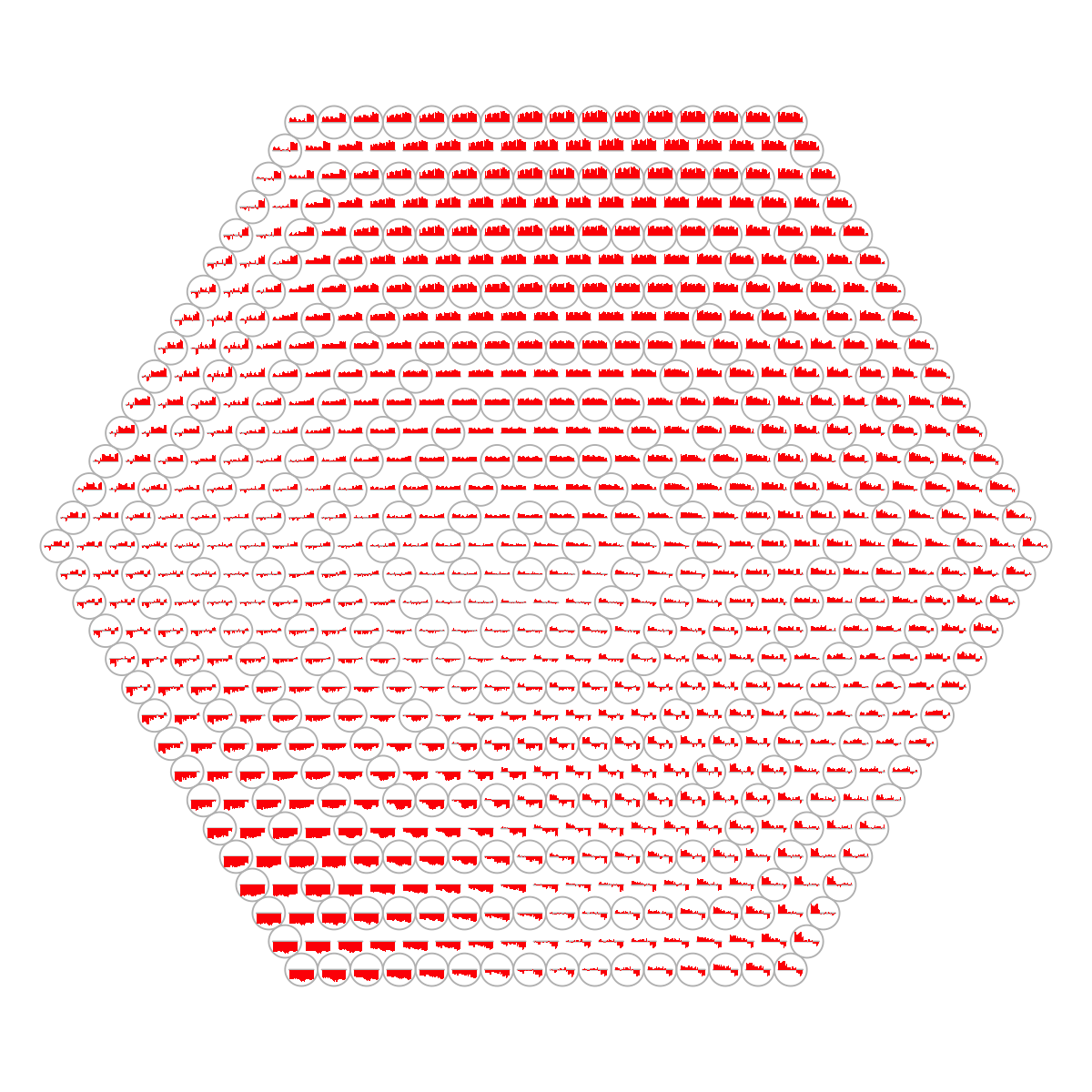
visHexPattern(sMap, plotType="lines")
## As you have seen, line plot displays the patterns associated with the codebook matrix. If multple colors are given, the points are also plotted. When the pattern involves both positive and negative values, zero horizental line is also shown.
visHexPattern(sMap, plotType="bars")
## As you have seen, bar plot displays the patterns associated with the codebook matrix. When the pattern involves both positive and negative values, the zero horizental line is in the middle of the hexagon; otherwise at the top of the hexagon for all negative values, and at the bottom for all positive values.
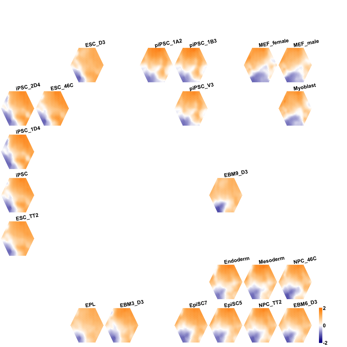
# (IV) Perform partitioning operation on the map to obtain continuous clusters (i.e. gene meta-clusters) as they are different from gene clusters in an individual map node
sBase <-
sDmatCluster(sMap)
 Start at 2016-06-24 11:45:30
First, define topology of a map grid (2016-06-24 11:45:30)...
Second, initialise the codebook matrix (63 X 22) using 'linear' initialisation, given a topology and input data (2016-06-24 11:45:30)...
Third, get training at the rough stage (2016-06-24 11:45:30)...
1 out of 638 (2016-06-24 11:45:30)
64 out of 638 (2016-06-24 11:45:30)
128 out of 638 (2016-06-24 11:45:30)
192 out of 638 (2016-06-24 11:45:30)
256 out of 638 (2016-06-24 11:45:30)
320 out of 638 (2016-06-24 11:45:30)
384 out of 638 (2016-06-24 11:45:30)
448 out of 638 (2016-06-24 11:45:30)
512 out of 638 (2016-06-24 11:45:30)
576 out of 638 (2016-06-24 11:45:30)
638 out of 638 (2016-06-24 11:45:30)
Fourth, get training at the finetune stage (2016-06-24 11:45:30)...
1 out of 2530 (2016-06-24 11:45:30)
253 out of 2530 (2016-06-24 11:45:30)
506 out of 2530 (2016-06-24 11:45:30)
759 out of 2530 (2016-06-24 11:45:30)
1012 out of 2530 (2016-06-24 11:45:30)
1265 out of 2530 (2016-06-24 11:45:30)
1518 out of 2530 (2016-06-24 11:45:30)
1771 out of 2530 (2016-06-24 11:45:30)
2024 out of 2530 (2016-06-24 11:45:30)
2277 out of 2530 (2016-06-24 11:45:31)
2530 out of 2530 (2016-06-24 11:45:31)
Next, identify the best-matching hexagon/rectangle for the input data (2016-06-24 11:45:31)...
Finally, append the response data (hits and mqe) into the sMap object (2016-06-24 11:45:31)...
Below are the summaries of the training results:
dimension of input data: 22x22
xy-dimension of map grid: xdim=9, ydim=7
grid lattice: rect
grid shape: sheet
dimension of grid coord: 63x2
initialisation method: linear
dimension of codebook matrix: 63x22
mean quantization error: 0.112148400297131
Below are the details of trainology:
training algorithm: sequential
alpha type: invert
training neighborhood kernel: gaussian
trainlength (x input data length): 29 at rough stage; 115 at finetune stage
radius (at rough stage): from 2 to 1
radius (at finetune stage): from 1 to 1
End at 2016-06-24 11:45:31
Runtime in total is: 1 secs
Start at 2016-06-24 11:45:30
First, define topology of a map grid (2016-06-24 11:45:30)...
Second, initialise the codebook matrix (63 X 22) using 'linear' initialisation, given a topology and input data (2016-06-24 11:45:30)...
Third, get training at the rough stage (2016-06-24 11:45:30)...
1 out of 638 (2016-06-24 11:45:30)
64 out of 638 (2016-06-24 11:45:30)
128 out of 638 (2016-06-24 11:45:30)
192 out of 638 (2016-06-24 11:45:30)
256 out of 638 (2016-06-24 11:45:30)
320 out of 638 (2016-06-24 11:45:30)
384 out of 638 (2016-06-24 11:45:30)
448 out of 638 (2016-06-24 11:45:30)
512 out of 638 (2016-06-24 11:45:30)
576 out of 638 (2016-06-24 11:45:30)
638 out of 638 (2016-06-24 11:45:30)
Fourth, get training at the finetune stage (2016-06-24 11:45:30)...
1 out of 2530 (2016-06-24 11:45:30)
253 out of 2530 (2016-06-24 11:45:30)
506 out of 2530 (2016-06-24 11:45:30)
759 out of 2530 (2016-06-24 11:45:30)
1012 out of 2530 (2016-06-24 11:45:30)
1265 out of 2530 (2016-06-24 11:45:30)
1518 out of 2530 (2016-06-24 11:45:30)
1771 out of 2530 (2016-06-24 11:45:30)
2024 out of 2530 (2016-06-24 11:45:30)
2277 out of 2530 (2016-06-24 11:45:31)
2530 out of 2530 (2016-06-24 11:45:31)
Next, identify the best-matching hexagon/rectangle for the input data (2016-06-24 11:45:31)...
Finally, append the response data (hits and mqe) into the sMap object (2016-06-24 11:45:31)...
Below are the summaries of the training results:
dimension of input data: 22x22
xy-dimension of map grid: xdim=9, ydim=7
grid lattice: rect
grid shape: sheet
dimension of grid coord: 63x2
initialisation method: linear
dimension of codebook matrix: 63x22
mean quantization error: 0.112148400297131
Below are the details of trainology:
training algorithm: sequential
alpha type: invert
training neighborhood kernel: gaussian
trainlength (x input data length): 29 at rough stage; 115 at finetune stage
radius (at rough stage): from 2 to 1
radius (at finetune stage): from 1 to 1
End at 2016-06-24 11:45:31
Runtime in total is: 1 secs
 Start at 2016-06-24 11:45:35
First, define topology of a map grid (2016-06-24 11:45:35)...
Second, initialise the codebook matrix (25 X 721) using 'linear' initialisation, given a topology and input data (2016-06-24 11:45:35)...
Third, get training at the rough stage (2016-06-24 11:45:35)...
1 out of 256 (2016-06-24 11:45:35)
26 out of 256 (2016-06-24 11:45:35)
52 out of 256 (2016-06-24 11:45:35)
78 out of 256 (2016-06-24 11:45:35)
104 out of 256 (2016-06-24 11:45:35)
130 out of 256 (2016-06-24 11:45:35)
156 out of 256 (2016-06-24 11:45:35)
182 out of 256 (2016-06-24 11:45:35)
208 out of 256 (2016-06-24 11:45:35)
234 out of 256 (2016-06-24 11:45:35)
256 out of 256 (2016-06-24 11:45:35)
Fourth, get training at the finetune stage (2016-06-24 11:45:35)...
1 out of 1000 (2016-06-24 11:45:35)
100 out of 1000 (2016-06-24 11:45:35)
200 out of 1000 (2016-06-24 11:45:35)
300 out of 1000 (2016-06-24 11:45:36)
400 out of 1000 (2016-06-24 11:45:36)
500 out of 1000 (2016-06-24 11:45:36)
600 out of 1000 (2016-06-24 11:45:36)
700 out of 1000 (2016-06-24 11:45:36)
800 out of 1000 (2016-06-24 11:45:36)
900 out of 1000 (2016-06-24 11:45:37)
1000 out of 1000 (2016-06-24 11:45:37)
Next, identify the best-matching hexagon/rectangle for the input data (2016-06-24 11:45:37)...
Finally, append the response data (hits and mqe) into the sMap object (2016-06-24 11:45:37)...
Below are the summaries of the training results:
dimension of input data: 8x721
xy-dimension of map grid: xdim=5, ydim=5
grid lattice: rect
grid shape: sheet
dimension of grid coord: 25x2
initialisation method: linear
dimension of codebook matrix: 25x721
mean quantization error: 2.13970227133359
Below are the details of trainology:
training algorithm: sequential
alpha type: invert
training neighborhood kernel: gaussian
trainlength (x input data length): 32 at rough stage; 125 at finetune stage
radius (at rough stage): from 1 to 1
radius (at finetune stage): from 1 to 1
End at 2016-06-24 11:45:37
Runtime in total is: 2 secs
Start at 2016-06-24 11:45:35
First, define topology of a map grid (2016-06-24 11:45:35)...
Second, initialise the codebook matrix (25 X 721) using 'linear' initialisation, given a topology and input data (2016-06-24 11:45:35)...
Third, get training at the rough stage (2016-06-24 11:45:35)...
1 out of 256 (2016-06-24 11:45:35)
26 out of 256 (2016-06-24 11:45:35)
52 out of 256 (2016-06-24 11:45:35)
78 out of 256 (2016-06-24 11:45:35)
104 out of 256 (2016-06-24 11:45:35)
130 out of 256 (2016-06-24 11:45:35)
156 out of 256 (2016-06-24 11:45:35)
182 out of 256 (2016-06-24 11:45:35)
208 out of 256 (2016-06-24 11:45:35)
234 out of 256 (2016-06-24 11:45:35)
256 out of 256 (2016-06-24 11:45:35)
Fourth, get training at the finetune stage (2016-06-24 11:45:35)...
1 out of 1000 (2016-06-24 11:45:35)
100 out of 1000 (2016-06-24 11:45:35)
200 out of 1000 (2016-06-24 11:45:35)
300 out of 1000 (2016-06-24 11:45:36)
400 out of 1000 (2016-06-24 11:45:36)
500 out of 1000 (2016-06-24 11:45:36)
600 out of 1000 (2016-06-24 11:45:36)
700 out of 1000 (2016-06-24 11:45:36)
800 out of 1000 (2016-06-24 11:45:36)
900 out of 1000 (2016-06-24 11:45:37)
1000 out of 1000 (2016-06-24 11:45:37)
Next, identify the best-matching hexagon/rectangle for the input data (2016-06-24 11:45:37)...
Finally, append the response data (hits and mqe) into the sMap object (2016-06-24 11:45:37)...
Below are the summaries of the training results:
dimension of input data: 8x721
xy-dimension of map grid: xdim=5, ydim=5
grid lattice: rect
grid shape: sheet
dimension of grid coord: 25x2
initialisation method: linear
dimension of codebook matrix: 25x721
mean quantization error: 2.13970227133359
Below are the details of trainology:
training algorithm: sequential
alpha type: invert
training neighborhood kernel: gaussian
trainlength (x input data length): 32 at rough stage; 125 at finetune stage
radius (at rough stage): from 1 to 1
radius (at finetune stage): from 1 to 1
End at 2016-06-24 11:45:37
Runtime in total is: 2 secs
)
)
)
)
)